


dead time
Double-pulse resolution, zero suppression, time-to-digital converter (TDC), time tagger, digitizer, DAQ, TCSPC, time-over-threshold, pile-up, SPAD, multi-hit
Dead time describes the time interval immediately following an event during which a measurement system (detector, discriminator, TDC, or high-speed ADC) cannot record or process subsequent signals. In time-resolved data acquisition, Time-of-Flight mass spectrometry (ToF-MS), and time-correlated single-photon counting (TCSPC), dead time can lead to systematic counting losses, spectral distortions, and limits the maximum throughput.
Due to dead time, the count rate actually measured by the system may be lower than the true rate of events striking the detector. To determine the true count rate in such a case, the detector’s dead-time behavior must be understood and corrected.
Fundamental Dead Time Models
In radiation detection and high-speed signal processing, dead time behavior follows two distinct mathematical models:
- Non-Paralyzable Model (Non-Extendable, also known as “Not-Updating-Dead-Time”):
Events arriving during the dead time τ are not detected and do not extend the dead time period. As soon as τ expires, the instrument is immediately ready to accept the next hit.
The relation between the true incoming event rate R and the measured rate m is:
m = R / (1 + R · τ) or R = m / (1 − m · τ)
At high event rates, the measured count rate asymptotically reaches a maximum saturation limit of m_max = 1/τ.
The digital logic, latches, and interpolation stages of a TDC are, by design, non-paralyzable. - Paralyzable Model (Extendable, also known as “updating dead time”):
Events arriving during an active dead time are lost and restart the dead time interval τ.
The observed count rate is governed by:
m = R · e(−R · τ)
If the input rate becomes too high (R >> 1/τ), the measured count rate drops dramatically, leading to complete system paralysis under high count-rate conditions.
In the entire measurement chain upstream of the TDC (detector and comparator/discriminator), behavior equivalent to an paralyzable dead time may occur at extremely high event rates.
Dead Time in Time-to-Digital Converters (TDCs)
In TDCs and Time Taggers, dead time characteristics are determined by front-end circuitry, buffer depth, and interface bandwidth:
- Channel-Specific Double-Pulse Resolution (Inter-Hit Dead Time): The minimum time required between two consecutive hits on the same channel to be recorded as separate time tags. In cronologic ASIC- and FPGA-based TDCs (e.g., xTDC4 and xHPTDC8-PCIe), the double-pulse resolution is down to a few nanoseconds.
- Independent Multi-Channel Processing (0 ns Inter-Channel Dead Time): Events arriving on separate physical channels do not block each other. Channels operate concurrently with zero cross-channel dead time.
- Multi-Edge & Time-over-Threshold (ToT): When capturing both leading and trailing edges (e.g., for pulse-height or time-walk compensation), the minimum detectable pulse width is defined by internal edge-transition switching times.
- Continuous Streaming with Zero Readout Dead Time: While legacy TDCs pause acquisition during conversion and readout cycles, cronologic streaming architectures utilize deep FIFOs to absorb event bursts and stream time tags continuously to host memory via PCIe DMA without measurement interruptions.
Dead Time in High-Speed ADCs and Digitizers
High-speed digitizers continuously sample incoming signals at multiple Gigasamples per second (GS/s). In these architectures, dead time is eliminated through high-throughput streaming and data reduction:
- Real-Time Zero Suppression: To prevent data congestion and buffer overflows when sampling continuously at 5 to 6.4 GS/s, cronologic Ndigo digitizers feature real-time FPGA-based zero suppression. The hardware streams only relevant signal windows exceeding a configurable threshold (along with pre- and post-trigger margins), discarding baseline noise without re-arm latency.
- Continuous PCIe DMA Streaming: Extracted waveform packets are transferred directly into host RAM at multiple Gigabytes per second, eliminating frame-to-frame acquisition pauses.
- Hardware Averaging: For repetitive signals, on-board FPGA averaging compresses data in real time, avoiding processing bottlenecks and dead-time-inducing CPU load.
System Integration: Detector Dead Time vs. Electronics Dead Time
Overall experiment dead time is a combination of detector physics and electronics performance:
- Detector Dead Time: SPAD quench and recharge cycles, MCP space charge saturation, photomultiplier tube (PMT) recharge dynamics, or scintillator luminescence decay.
- Electronics Dead Time: Discriminator recovery, TDC double-pulse resolution, FIFO buffers, and bus transfer limits.
The selection of suitable detectors with the shortest possible dead time therefore plays a crucial role. This is because, as mentioned above, at extremely high event rates, effects can occur in the measurement chain that correspond to a paralyzable dead time:
- The signal remains above the switching threshold: A signal transition is mandatory for the TDC to trigger a timestamp creation. If detector pulses have a finite decay time (fall time) and another pulse arrives before the signal has fallen below the comparator threshold again, the comparator output remains high continuously. If many pulses follow one another in rapid succession, the signal remains permanently above the threshold—the system thus no longer generates new edges and becomes blocked (paralysis effect).
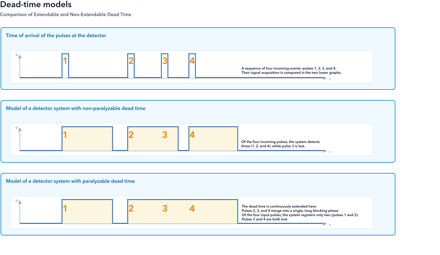
Dead-Time behavior in signal acquisition: Comparison of extendable and non-extendable dead time.
In the second graph, pulse 1 arrives and is registered by the system, triggering a dead time of fixed duration τ. This is represented here by the yellow box. Since the dead time has already elapsed completely before pulse 2 arrives, it is also successfully registered and starts a new dead-time interval τ. pulse 3, on the other hand, arrives while the dead time from pulse 2 is still active. In the non-extendable model, pulse 3 is therefore simply ignored and discarded. Since the dead time has elapsed before pulse 4 arrives, it is subsequently registered as an event in the usual manner.
In the third graph, pulse 1 arrives, is registered, and starts the dead time τ. Once τ has elapsed, the system is ready again, so pulse 2 is also registered and a new dead time begins. pulse 3 arrives during this ongoing dead time as well. Although pulse 3 is not counted, it completely resets the dead time interval τ at the moment of its arrival. Even before this extended interval can expire, pulse 4 arrives and also resets the dead time.